Geospatial Accuracy
Background
The complex image output of the SAR image-formation process is a set of focused pixels with phase and amplitude values. Each pixel pair of the image is referenced to the sensor by its range and azimuth coordinates. That is, each pair has a specific range to a sensor reference location and an azimuth location in the along-track direction. This range-azimuth geometry establishes an arc in space, which is the basis of the geolocation modeling of SAR images. The arc for each pixel is initially fit to the slant plant surface, and for amplitude images it is subsequently projected to a ground surface, such as the ground plane or ellipsoid or topographic surface. The geolocation accuracy of an image depends on how well that range-azimuth arc is measured. The relevant parameters for the arc are: the range and azimuth values, the sensor reference location, and the sensor velocity vector. We will consider each of them in turn.
Range
A SAR system is able to measure the range to a point on the ground very precisely. The theoretical precision of range is a fraction of a wavelength. However, as the RADAR pulse propagates through the atmosphere, it undergoes diffraction which curves the path of the pulse. This adds an unintended increase to the range of an object. The amount of increase depends on the look angle, the location of the satellite and scene, and even the time of day. The ICEYE SAR processor applies path length corrections (typically on the order of a couple of metres) using well established models.
Azimuth
The sensor also compares pulses to measure how the range to a point changes as the satellite moves along its trajectory. This provides precise information of the azimuth, or along-track, location of a pixel. Since this record is derived from precise pulse-to-pulse phase changes, it is the most accurate aspect of SAR data.
On-Board Timing Errors
A fundamental source of error for all RADAR systems relates to timing. In radar systems, precise electronic clocks are used to record the passage of time. All clocks have some sort of drift in their accuracy which, if not corrected, affects the measured range and focussing of the imagery. ICEYE satellites apply timing corrections to their internal clocks by periodically synchronising with GNSS (Global Navigation Satellite System) satellites.
Orbit Knowledge
A potentially large source of errors comes from not knowing precisely where the sensor is when each pulse is transmitted and received. This is determined by the satellite's orbit knowledge. ICEYE satellites constantly record their GNSS location. This information is transmitted to the ground during ground station telemetry downloads that occur usually once per orbit (sometimes more frequently). Additionally, the GNSS data is stored with the wideband radar data for rapid downlink and processing.
Once on the ground, the orbit information is passed to ICEYE's orbit determination servers. These refine the orbit by taking into account the satellite's attitude and motion, the solar radiation pressure and the local gravitational field strength. The refinements are then used to improve the image geospatial accuracy and to provide accurate time/position/velocity estimates for future collections.
In the future we plan on further refining the orbit fidelity using post-collected GNSS corrections combined with retroreflectors attached to the satellite.
The Following table summarises the different levels of orbit fidelity. This information is stored in each image's metadata.
| ORBIT FIDELITY | DESCRIPTION | LATENCY |
|---|---|---|
| Predicted | Uses the latest orbit solution to predict where the satellite will be at some point in the future. It is used for collection planning and feasibility studies. It is not typically used for image formation processing because it has the largest errors. | updated 6 hours before collection |
| Rapid | Uses GNSS stored samples collected during or near to the imaging operation. The spherical error (SE90) of the samples is 3 m. This allows imagery to be downlinked during or soon after collection to provide tactical SAR imagery to users with a modest geospatial error. This level is not yet available on all satellites. | Immediate |
| Precise | This is the default orbit fidelity used for ICEYE satellites. The satellite position and velocity state vectors are refined after the imaging operation using downlinked telemetry and attitude data. The spherical error of the refined data is 1.5 m | 10-45 minutes after imaging operation |
| Scientific | This uses GNSS corrections applied to the samples taken during imaging to significantly reduce the position velocity error. This is not yet available across the ICEYE Fleet. | 2 to 4 days after collection |
Orbit Knowledge Metadata
The location of the satellite during any imaging operation is made available by including the satellite and velocity information in the metadata for each image product. The data can be found under the orbit_state_vector metadata element. The accuracy of each element is determined by the orbit fidelity used to create the product which can be found in the orbit_processing_level metadata element which corresponds so one of the levels in table 1.
Determining Ground Locations
A sensor-orientation SAR amplitude image is a distillation of its richer complex image parent. It is the viewable version of SAR pixels and thus contains only microwave brightness values and no phase data. As with the complex image, its pixels have a range-azimuth structure. The difference is that it is usually projected to a ground surface, not the slant plane. It must be emphasized that the SAR image on its own cannot provide accurate ground locations. The chosen ground projection surface is typically an ellipsoid with a height set to the average height of the imaged area. This means that latitude and longitude image corner coordinates are for reference only. They are intended to layout the image footprint, and since they were projected to a single-elevation surface they cannot be used for accurate geolocation. SAR geolocation requires the projection of the natural range-azimuth arc of each pixel to an actual terrain height. This means that the image exploitation system must have a ground terrain height model on hand and it must use the coded SAR geometry model equations. This situation is exactly the same for optical images. The imaging conversion of 3D space to any 2D image, optical or SAR, means that proper geolocation requires pixel projections to elevation models on exploitation workstations.
Elevation Models
In the case of a calibrated SAR with accurate range-azimuth coordinates and precise orbit data, the most significant source of geospatial error comes from the way the data is measured and exploited on a workstation. The following animation explains why the measured location of a point on an accurate SAR image is dominated by errors in external terrain height information.
The Geolocation Potential of SAR
It is interesting to consider the pristine potential of SAR geolocation. Both SAR and optical satellite sensors can provide accurate orbit information, but optical sensors also need to physically measure the pointing orientation of the sensor to the ground. These data are derived from on-board gyroscopes and star sensors, and errors in the estimates of the sensor pointing direction project along the huge distance to the ground surface. A SAR satellite must also estimate pointing direction in order to illuminate the proper location on the ground. But once the image is formed, the angle to the ground location is determined by the azimuth coordinate, which is itself derived from ultra-precise pulse-to-pulse phase changes. The aspect of optical geolocation which contributes the most uncertainty, pointing direction, is not a significant factor for SAR geolocation. A well-calibrated SAR with accurate orbits, in conjunction with precise elevation data, can provide a geolocation accuracy of less than one meter for well-defined points. This is the precision to which ICEYE aspires.
Geospatial Metadata
It is interesting to note that the ground projection issue relates to any oblique looking imaging system (such as optical sensors) that are able to take images off-nadir. Fortunately a lot of geospatial viewers and exploitation tools have evolved to help the user deal with such issues. Some viewers have terrain models built in and can provide precise location information using parameters embedded in the metadata of each image. Two common approaches are Doppler Centroid Polynomials and Rapid Polynomial Coefficients.
Fast and Simple Geolocation: Rapid Positioning Capability
The range-azimuth arc and its associated geometry model equations form the rigorous, physics-based foundation of SAR geolocation. However, the actual implementation of this model is quite detailed and can include ponderous and slow iterative solutions. An engineering replacement to optical and SAR physics-based geometry models is commonly used to speed and simplify the calculation of ground locations. This replacement model takes the form of a ratio of polynomials that link a ground location (in latitude, longitude and height) to its associated image location. The replacement engineering model has been called Rational Polynomial Coefficients (RPC), but at ICEYE we prefer to call it Rapid Positioning Capability. The latter term instantly indicates its purpose and value, rather than referencing its mathematical structure. Because it is merely a polynomial replacement, the RPC data structure provided for ICEYE SAR images is exactly the same as the RPC model for all optical images. RPC is not only fast and simple; it is also sensor- and phenomenology-independent.
It should be noted that RPC data are derived from an image’s geometric metadata and the physics-based geometry model for that sensor. They are usually calculated during image formation and included in the output image file. RPC coefficients are provided for ICEYE’s amplitude images in the GRD format. The model is described in [ 1 ] which extends the work for the National Imagery Transmission Format (NITF)2 to GeoTIFFs. The translation of latitude, longitude and height to image pixel coordinates is described below.
The approximation used in ICEYE products is a set of rational polynomials that describe the normalized row and column values (\(rn\) , \(cn\)) as a function of normalized geodetic latitude, longitude, and height. The link between the two is the (\(P\), \(L\), \(H\)) set of normalized polynomial coefficients (LINE_NUM_COEF_n, LINE_DEN_COEF_n, SAMP_NUM_COEF_n, SAMP_DEN_COEF_n) as applied in the RPC polynomial format. Normalized values, rather than actual values are used in order to minimize the introduction of errors during the calculations. The transformation between row and column values (\(r\),\(c\)) and normalized row and column values (\(r_n\), \(c_n\)), and between the geodetic latitude, longitude, and height ( φ, λ, h ), and normalized geodetic latitude, longitude, and height (P, L, H) is defined by a set of normalizing translations (offsets) and scales that ensure all values are contained within the range -1 to +1. The normalization of these parameters is given in Table 2.
If you load ICEYE's images into RPC-compliant GIS Viewers (eg QGIS3), with access to a ground elevation model, the Viewer will automatically perform conversion from image row, column to lat, long, height (WGS84 geoid).
| NORMALISED | DEFINITION |
|---|---|
| \(P\) | (Latitude - LAT_OFF) / LAT_SCALE |
| \(L\) | (Longitude - LONG_OFF) / LONG_SCALE |
| \(H\) | (Height - HEIGHT_OFF) / HEIGHT_SCALE |
| \(r_n\) | (Row - LINE_OFF) / LINE_SCALE |
| \(c_n\) | (Column - SAMP_OFF) / SAMP_SCALE |
The GeoTIFF encoding of the RPC data in ICEYE data products is provided as a structure of 14 parameters described in Table 3.
The equation to calculate the row and column number from the RPC values is given by:
Where the rational polynomial numerators and denominators are each a 20-point cubic polynomial function of the form:
| RPC CUBIC POLYNOMIAL | ||||
|---|---|---|---|---|
| \(\sum_{i=1}^{20} C_i ⋅ \rho_i(P,L,H) =\) | ||||
| \(C_1\) | \(+C_6 LH\) | \(+C_{11} PLH\) | \(+C_{16} P^3\) | |
| \(+C_2L\) | \(+C_7 PH\) | \(+C_{12} L^3\) | \(+C_{17} PH^2\) | |
| \(+C_3P\) | \(+C_8 L^2\) | \(+C_{13} LP^2\) | \(+C_{18} L^2 H\) | |
| \(+C_4H\) | \(+C_9 P^2\) | \(+C_{14} LH^2\) | \(+C_{19} P^2 H\) | |
| \(+C_5LP\) | \(+C_{10} H^2\) | \(+C_{15} L^2P\) | \(+C_{20} H^3\) |
Where coefficients \(C_1…C_{20}\) represent the vector coefficients provided in the product metadata : LINE_NUM_COEF_n, LINE_DEN_COEF_n, SAMP_NUM_COEF_n, SAMP_DEN_COEF_n. The image coordinates are in units of pixels. The ground coordinates are latitude and longitude in units of decimal degrees and the height above ellipsoid is in units of meters. The ground coordinates are referenced to WGS84.
| NAME | DESCRIPTION | VALUE RANGE | UNITS |
|---|---|---|---|
| LINE_OFF | Line Offset | >= 0 | pixels |
| SAMP_OFF | Sample Offset | >= 0 | pixels |
| LAT_OFF | Geodetic Latitude Offset | -90 to +90 | degrees |
| LONG_OFF | Geodetic Longitude Offset | -180 to +180 | degrees |
| HEIGHT_OFF | Geodetic Height Offset | unlimited | meters |
| LINE_SCALE | Line Scale | > 0 | pixels |
| SAMP_SCALE | Sample Scale | > 0 | pixels |
| LAT_SCALE | Geodetic Latitude Scale | 0 < LAT_SCALE <= 90 | degrees |
| LONG_SCALE | Geodetic Longitude Scale | 0 < LONG_SCALE <= 180 | degrees |
| HEIGHT_SCALE | Geodetic Height Scale | HEIGHT_SCALE > 0 | meters |
| LINE_NUM_COEFF (1-20) | Line Numerator Coefficients. Twenty coefficients for the polynomial in the Numerator of the \(r_n\) equation. | unlimited | |
| LINE_DEN_COEFF (1-20) | Line Denominator Coefficients. Twenty coefficients for the polynomial in the Denominator of the \(r_n\) equation. | unlimited | |
| SAMP_NUM_COEFF (1-20) | Sample Numerator Coefficients. Twenty coefficients for the polynomial in the Numerator of the \(c_n\) equation. | unlimited | |
| SAMP_DEN_COEFF (1-20) | Sample Denominator Coefficients. Twenty coefficients for the polynomial in the Denominator of the \(c_n\) equation. | unlimited |
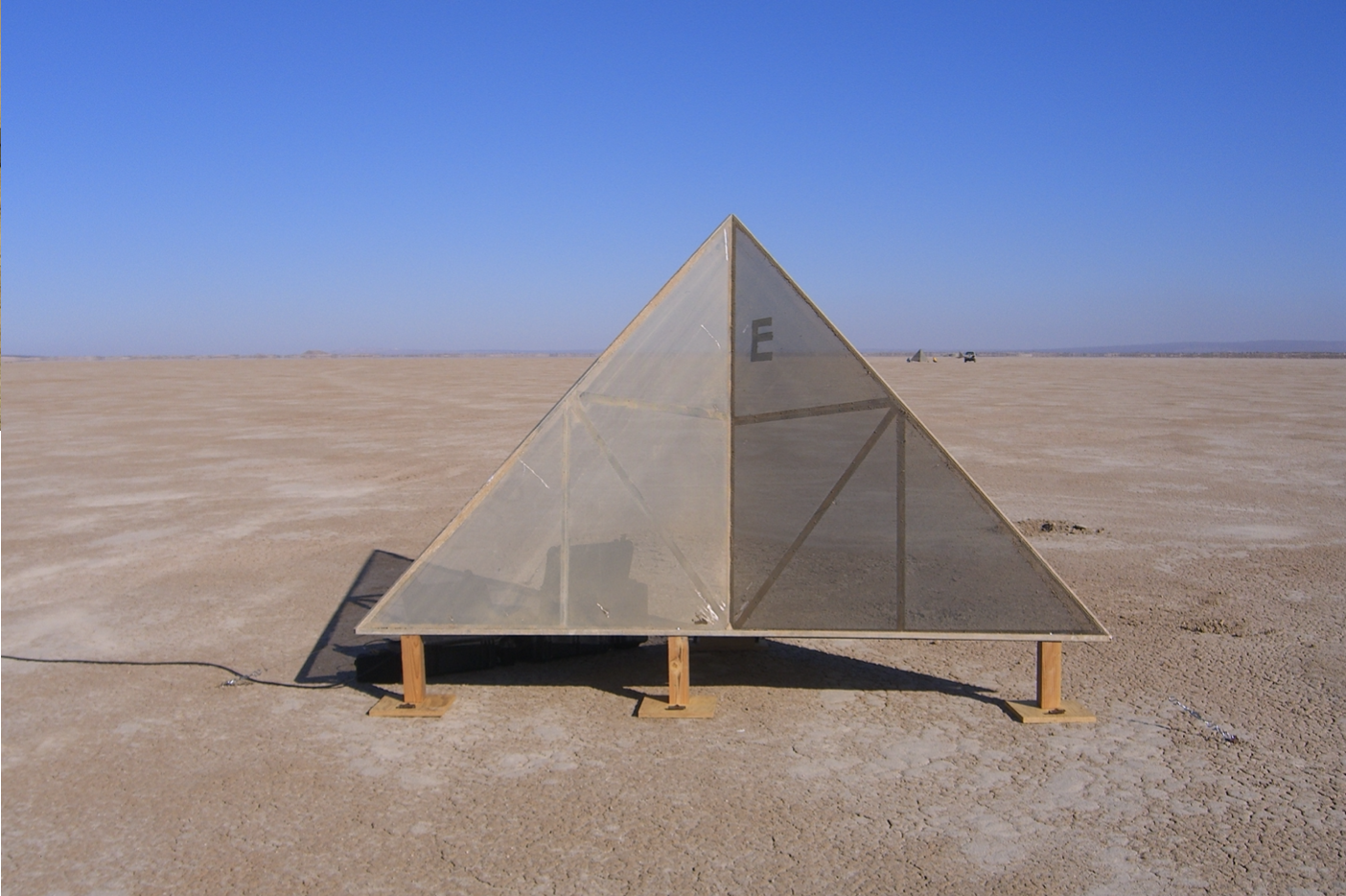
Geometric Calibration Process
In order to monitor the geometric integrity of ICEYE images, the satellites routinely collect images over ground-surveyed calibration sites around the world. Each site consists of a set of calibration point targets such as trihedral corner reflectors. The position, orientation and size of these features are carefully measured and maintained, and they are often provided by organizations such as NASA JPL as a free service to the geospatial community. ICEYE engineers compare the target ground coordinates derived from the image coordinates and known elevation to the precisely surveyed ground-truth coordinates. These calibration comparisons provide a statistical measure of the horizontal accuracy of ICEYE images by comparing calibration point target locations in terrain corrected imagery to ground truth measurements of each calibration point target. The root, mean square error (RMSE) is then calculated from all the measured location errors. Currently the ICEYE fleet is achieving a worst-case RMSE of 6 m. In actual practice elevation models used during image exploitation have vertical uncertainties, and feature signatures are not as precise as those of corner reflectors. Together these increase the horizontal error of image-derived ground coordinates.
References
-
OSGeo. RPCs in GeoTIFF. URL: http://geotiff.maptools.org/rpc_prop.html. ↩
-
National Imagery and Mapping Agency. The Compendium of Controlled Extensions \(CE\) for the National Imagery Transmission Format \(NITF\) Version 2.1. November 2000. URL: http://geotiff.maptools.org/STDI-0002_v2.1.pdf. ↩
-
QGIS - A Free and Open Geographic Information System. Accessed 2020 Dec 17. URL: https://qgis.org/en/site/. ↩
-
R.J. Muellerschoen. The rosamond corner reflector array for sar calibration; past, present, future. 7th Nov 2017. Accessed 30 December 2021. URL: https://trs.jpl.nasa.gov/handle/2014/48764. ↩