Range Resolution
Fixing Range Resolution by Synthesizing a Short Pulse
In our discussions about aperture synthesis, we did not say anything about range resolution. This is because the “synthetic aperture” technique itself deals only with azimuth. It does not do anything to address the problem we saw with brute-force range resolution. Recall that this is one-half of the pulse length, which is the speed of light (\(c\)) times the pulse duration, \(T\):
where \(\delta_{ra}\) is the slant range resolution.
Thus far, we have described our radar pulses as if they have a fixed frequency, like X-band pulses of 10 GHz frequency and a 3 cm wavelength. But most radars actually transmit chirped pulses in which the frequency changes (Figure 11). Notice how the wavelength of the green pulse is manipulated and varies from long to short
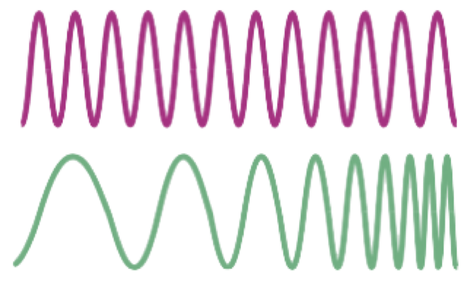
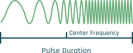
When we state the frequency or wavelength of a SAR sensor, those values typically apply at the mid-way time of the pulse. This is known as the radar center frequency or wavelength. The actual transmitted wavelengths are varied quite a bit on either side to form chirped pulses (Figure 12).
There are many different pulse modulation techniques, but the chirp with a smoothly varying frequency is most common. A chirped pulse is easy to produce and since the total transmitted energy is a product of amplitude and duration, a long pulse can contain a substantial amount of energy without needing a large peak power.
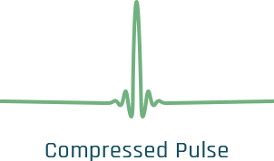
A chirped pulse enables high range resolution because its form is exactly specified and its echo is a reversed and weakened copy. The reflection has the same shape as the emitted signal, it’s just flipped and has a much smaller amplitude. The two are compared in what is called a matched filter process. The known structure of the emitted pulse is compared to the echo at various locations. A calculation is performed, and if they are misaligned the result of this calculation is zero. At the exact location where they match there is a strong signal that indicates the match. A synthetic pulse that is narrow in range replaces the spread-out pulse (Figure 13).
The width of the compressed pulse is based entirely on the bandwidth of the emitted pulse. The slant range resolution equation is transformed:
This is a really beautiful equation. It is so simple and powerful. Resolution in range is entirely based on how much bandwidth we impart to chirped pulses, and like its azimuth counterpart it has nothing whatsoever to do with distance to the ground.
Slant Range Resolution Examples
So how much can we vary pulse frequency? Well, bandwidths can be made really large. Consider an X-band system capable of 300,000,000 cycles per second (300 MHz) of bandwidth. We can calculate resolution in the slant range:
Plans for the next generation of ICEYE satellites include pulse bandwidths of 600 MHz and 1200 MHz. These will yield a slant range resolution cell of 0.25 meters and better from a satellite that is perhaps 750,000 meters away from the imaged area.
Ground Range Resolution
The slant range is the distance between the antenna and the target, and that is the direction where range resolution is measured. To produce images along the ground surface, the pixels have to be projected to the “ground range” from their original slant range orientation (Figure 14). This has the effect of elongating the pixels in range.
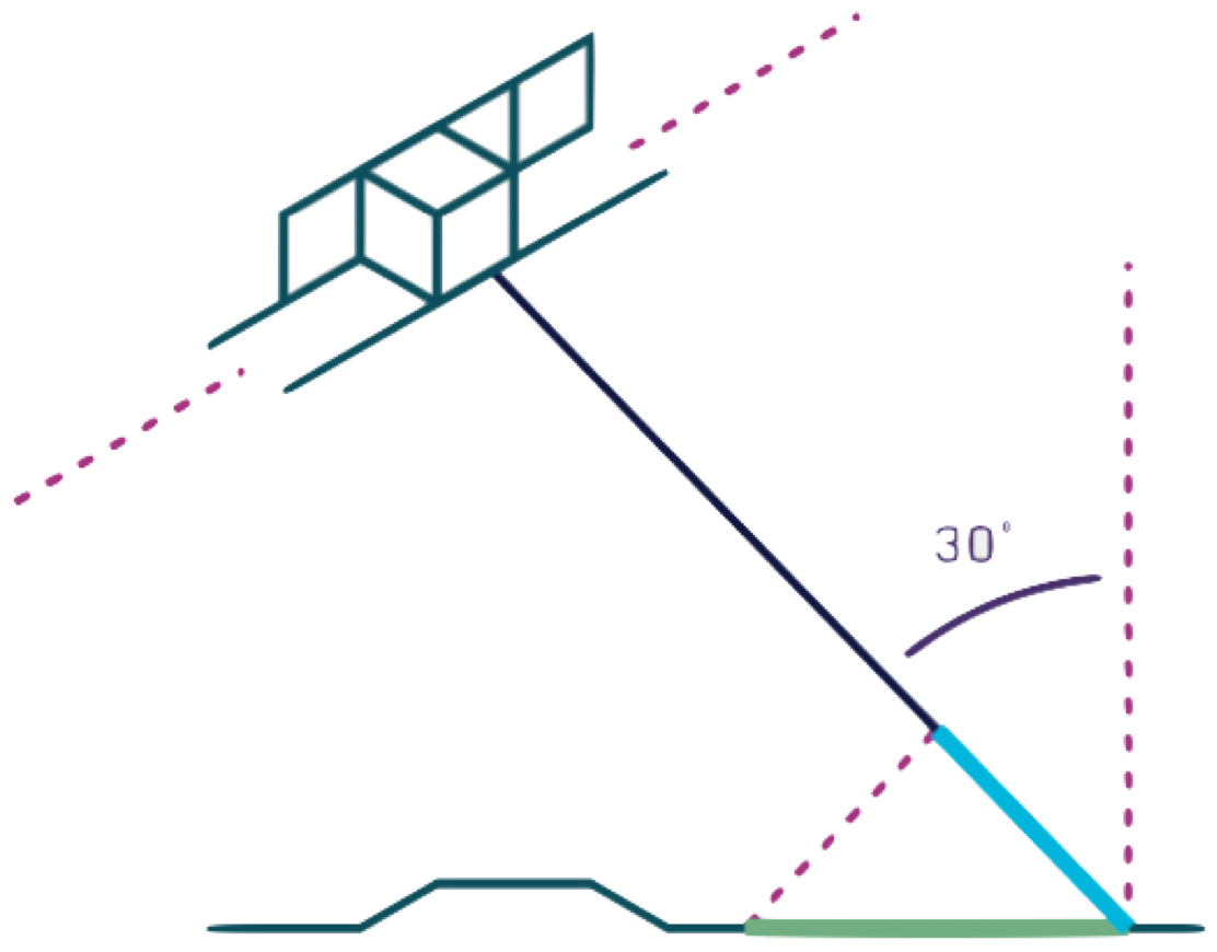
The illustration shows the relationship between slant range resolution, shown in blue, and the length of the equivalent resolution distance along the ground, shown in green. When the illumination is steep, as in this example, the projection to the ground surface results in a much longer ground range cell. You can imagine what would happen as the steepness continued to approach nadir. This is exactly opposite to the situation with optical imaging resolution, which is best at nadir.
Slant range and ground range resolution comparisons for two incidence angles are shown in Table 2. Notice the dramatic increase for the steeper illumination.
| INCIDENCE ANGLE 30° | INCIDENCE ANGLE 60° | |
|---|---|---|
| Slant Range | 0.50m | 0.50m |
| Ground Range | 1.00m | 0.55m |
While slant range resolution seems “better” than ground range resolution, keep in mind that it refers to the sensor’s ability to discriminate features along the oblique path of the energy. Most of the features we care about lie along the ground surface, and ground range resolution is a useful way to describe image resolution.